|
|
Class documentation of Concepts
We present a very terse introduction into the basic classes and the mathematical ideas. This is also available on a color poster which prints nicely in A0-A4.
Concept Oriented Design
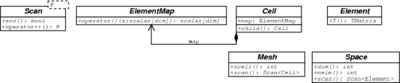
The numerical methods which should be implemented are already formulated in an abstract way based on hierarchical structured mathematical concepts. Therefore, represent each concept by a module and combine the modules according to the numerical algorithm. This defines concept oriented design.
Mathematical Concepts | Fundamental Classes |
Find
Find
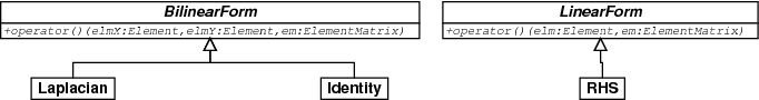
Using a basis | Bilinear form Mesh |
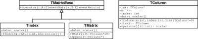
Assembling using T matrices: ![$\left . \Phi_i \right |_K = \displaystyle \sum_{j=1}^{m_K} [\boldsymbol
T_K]_{ji} \phi_j^K$](form_255_dark.png)
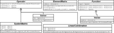
| Assembling the global matrix and the load vector and solving the linear system: The T matrices are built columnwise: each column in a T matrix corresponds to a global degree of freedom: |
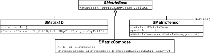
The constraints of hanging nodes are eliminated using S matrices: ![$\left . \phi_j^K \right |_{K'} = \displaystyle
\sum_{l=1}^{m_{k'}} [\boldsymbol S_{K' K}]_{lj} \phi_l^{K'}$](form_258_dark.png)    | S matrices in 1D are computed by solving a linear system. In higher dimensions, tensor product and composition is used:  (large) (large) |


![\[\underbrace{\int_\Omega \nabla u \cdot \nabla v \, dx +
\int_\Omega u v \, dx}_{=: a(u,v) \text{ bilinear form}} =
\underbrace{\int_\Omega f v \, dx + \int_{\Gamma_N} g_N v \,
ds}_{=: l(v) \text{ linear form}}.\]](form_243_dark.png)


![\[a(u,v) = l(v).\]](form_246_dark.png)


![$[\boldsymbol A]_{ij} = a(\Phi_i, \Phi_j)$](form_249_dark.png)
![$[\vec l]_i = l(\Phi_i)$](form_250_dark.png)


![\[ \vec l = l(\vec \Phi) = \sum_{\tilde K} \boldsymbol T_{\tilde
K}^\top l(\vec \phi^{\tilde K}) = \sum_{\tilde K} \boldsymbol T_{\tilde
K}^\top \vec l_{\tilde K} \]](form_256_dark.png)
![\[ \boldsymbol A = a(\vec \Phi, \vec \Phi) = \sum_{K, \tilde K} \boldsymbol
T_{\tilde K}^\top a(\vec \phi^K, \vec \phi^{\tilde K}) \boldsymbol T_K =
\sum_{K, \tilde K} \boldsymbol T_{\tilde K}^\top \boldsymbol A_{\tilde K K}
\boldsymbol T_K \]](form_257_dark.png)
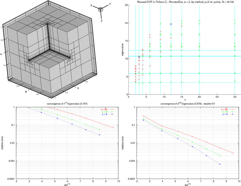
Result: Exponential Convergence
Solving the Maxwell Eigen value problem in a perfect conductor boundary condition domain 

- See also
- [1] M. Costabel, M. Dauge. Weighted regularization of Maxwell equations in polyhedral domains. Numer. Math. 93(2) (2002) 239-277.
Generated on Wed Sep 13 2023 21:06:25 for Concepts by