|
|
Class documentation of Concepts
Contents
@section intro Introduction
In this tutorial the implementation of inhomogeneous Dirichlet boundary
conditions using a Dirichlet lift ansatz is shown.

The equation solved is the reaction-diffusion equation
\f[ - \Delta u + u = f \f]
in the unit square \f$ \Omega = (0,1)^2 \f$ with source term
\f[
f(x,y) = -5\exp\left(-(x-1/2)^2-(y-1/2)^2\right)
\f]
and Dirichlet boundary conditions
\f[
u =
\begin{cases}
\sin \pi x, &(x,y)\in\Gamma_{\rm inh}=\{(x,y)\in\partial\Omega\mid y=0\},\\
0,          &(x,y)\in\partial\Omega\setminus\Gamma_{\rm inh}.
\end{cases}
\f]

A suitable Dirichlet lift is
\f[ g = \sin \pi x \; \cos \frac{\pi}{2} y. \f]
By setting \f$ u = \tilde{u} + g \f$ the reaction-diffusion equation simplifies
to a problem in \f$ \tilde{u} \f$
\f[
- \Delta \tilde{u} + \tilde{u} = f + \Delta g - g, \qquad x\in\Omega,
\f]
with homogeneous Dirichlet boundary conditions
\f[
\tilde{u} = 0, \qquad x\in\partial\Omega.
\f]

@section variation Variational Formulation
Now we derive the corresponding variational formulation of the introduced problem:
find \f$ \tilde{u}\in H^1_0(\Omega) \f$ such that
\f[
\int_{\Omega}\nabla\tilde{u}\cdot\nabla v\;{\rm d}x
+ \int_{\Omega}\tilde{u}v\;{\rm d}x
=
\int_{\Omega}fv\;{\rm d}x
-\int_{\Omega}\nabla g\cdot\nabla v\;{\rm d}x
- \int_{\Omega}gv\;{\rm d}x \qquad\forall v\in H^1_0(\Omega).
\f]

@dontinclude inhomDirichletBCs.cc
@section commented Commented Program
First, system files
@until iostream
and concepts files
@until toolbox
are included. With the following using directive
@until using
we do not need to prepend <tt>concepts::</tt> to <tt>Real</tt> everytime.

@subsection main Main Program
The mesh is read from three files containing the coordinates, the
elements and the boundary attributes of the mesh.
@until endl
<!--Please see the tutorial @ref mesh "Import 2D Mesh" for a concise explanation of how to write these import files and define the attributes for edges etc. -->
In our example the edges are given the following attributes: 1 (bottom), 2 (right), 3 (top) and 4 (left).

Now the mesh is plotted using a scaling factor of 100, a greyscale of 1.0
and one point per edge.
@until drawMeshEPS

The Dirichlet lift and its gradient are defined.
@skip concepts
@until DirichletLiftGrady

The problem for \f$ \tilde{u} \f$ has homogeneous Dirichlet boundary conditions at
all four edges.
@skip concepts
@until bc.add

Using the mesh and the homogeneous Dirichlet boundary conditions, the space
can be built. We refine the space two times and set the polynomial degree to three.
Then the elements of the space are built and the space is plotted.
@skip hp2D
@until drawMeshEPS

The right hand side is computed, containing the integrals of the source term,
the Dirichlet lift and its gradient.
@skip hp2D
@until endl

The system matrix is computed from the bilinear form \c hp2D::Laplace<Real> and
the bilinear form \c hp2D::Identity<Real>.
@skip hp2D
@until endl

We solve the equation using the conjugate gradient method with a tolerance of
1e-6 and a maximum number of iterations of 200.
@skip concepts
@until endl

In order to add the Dirichlet lift to the solution of the homogeneous Dirichlet
problem we transform the solution, that is given as a vector related to the basis
functions of \c spc, into an element formula, that can be evaluated at each point
in every cell.
@skip concepts
@until endl

We plot the solution, the homogeneous Dirichlet solution and the Dirichlet lift
using <tt>graphics::MatlabGraphics</tt>. To this end the shape functions are
computed on equidistant points using the trapezoidal quadrature rule.
@skip hp2D
@until MatlabGraphics
@until MatlabGraphics
@until MatlabGraphics

Finally, exceptions are caught and a sane return value is given back.
@until }
@until }

@section results Results
Output of the program:
@code
Mesh: Import2dMesh(ncell = 1)
RHS Vector: Vector(121, [-7.813458e-01, -1.331759e-01, -1.446913e-04, -8.977796e-02, -1.975711e-02, -1.504745e-02, -1.103641e-04, -3.490666e-03, 4.167881e-05, -1.009906e+00, -1.735826e-01, 3.466376e-04, -1.628611e-01, 8.126026e-03, -2.796551e-02, 4.594644e-05, -1.436936e-03, 1.759809e-05, -8.586824e-01, -6.786590e-01, -1.598694e-01, 5.110721e-03, -1.388192e-01, -6.395889e-03, -1.248594e-01, -3.466673e-03, -2.580936e-02, 8.124231e-04, -1.244348e-03, 5.860425e-05, -8.122847e-02, -1.558898e-02, -1.461248e-02, 2.876690e-04, -3.028574e-03, 1.411786e-04, -7.813458e-01, -1.331759e-01, -1.446913e-04, -1.628611e-01, 8.126026e-03, -2.796551e-02, 4.594644e-05, 1.436936e-03, -1.759809e-05, -8.977796e-02, -1.975711e-02, -1.504745e-02, -1.103641e-04, 3.490666e-03, -4.167881e-05, -6.786590e-01, -8.122847e-02, -1.558898e-02, -1.248594e-01, -3.466673e-03, -1.461248e-02, 2.876690e-04, 3.028574e-03, -1.411786e-04, -1.388192e-01, -6.395889e-03, -2.580936e-02, 8.124231e-04, 1.244348e-03, -5.860425e-05, -4.822921e-01, -5.869802e-01, -9.922001e-02, 6.668103e-03, -9.533732e-02, 3.713134e-03, -1.236099e-01, -9.222017e-03, -2.002021e-02, 1.475922e-03, 8.660092e-04, -9.094635e-05, -6.180870e-02, -9.103448e-03, -1.221454e-02, 6.601945e-04, 2.115183e-03, -2.198685e-04, -6.016121e-02, -8.736539e-03, -8.218690e-03, 9.139240e-04, 8.895484e-04, -2.644021e-04, -7.032423e-02, -1.180407e-02, -1.147942e-02, 1.894019e-03, 3.595180e-04, -1.091848e-04, -4.822921e-01, -9.922001e-02, 6.668103e-03, -6.180870e-02, -9.103448e-03, -1.221454e-02, 6.601945e-04, -2.115183e-03, 2.198685e-04, -9.533732e-02, 3.713134e-03, -2.002021e-02, 1.475922e-03, -8.660092e-04, 9.094635e-05, -6.016121e-02, -8.736539e-03, -1.147942e-02, 1.894019e-03, -3.595180e-04, 1.091848e-04, -8.218690e-03, 9.139240e-04, -8.895484e-04, 2.644021e-04])
System Matrix: SparseMatrix(121x121, HashedSparseMatrix: 1521 (1.038863e+01%) entries bound.)
Solver: CG(solves SparseMatrix(121x121, HashedSparseMatrix: 1521 (1.038863e+01%) entries bound.), eps = 6.210533e-13, it = 37, relres = 0)
Solution: FrmE_Sum(ElementFormulaVector<1>(hp2D::Value<double>(), Vector(121, [-5.387654e-01, -3.006218e-01, 1.564124e-02, -1.425659e-01, -4.809499e-03, -1.088256e-01, 1.611971e-02, 8.625588e-03, -6.891406e-03, -7.373583e-01, -4.048944e-01, 1.925875e-02, -1.941122e-01, 2.767690e-03, -1.016416e-01, 3.259733e-03, -1.569518e-03, 2.857100e-04, -8.461932e-01, -6.183710e-01, -2.393483e-01, 9.380839e-03, -2.230022e-01, -2.981412e-03, -1.722831e-01, -6.882467e-03, -6.528885e-02, 2.490903e-03, -1.108972e-03, -1.050398e-05, -1.618117e-01, -6.560393e-03, -3.530271e-02, 1.727733e-03, -4.305751e-03, 3.179923e-04, -5.387655e-01, -3.006218e-01, 1.564124e-02, -1.941122e-01, 2.767687e-03, -1.016416e-01, 3.259733e-03, 1.569518e-03, -2.857100e-04, -1.425659e-01, -4.809502e-03, -1.088256e-01, 1.611971e-02, -8.625588e-03, 6.891407e-03, -6.183710e-01, -1.618117e-01, -6.560394e-03, -1.722831e-01, -6.882469e-03, -3.530271e-02, 1.727733e-03, 4.305752e-03, -3.179924e-04, -2.230022e-01, -2.981412e-03, -6.528885e-02, 2.490903e-03, 1.108972e-03, 1.050400e-05, -4.161721e-01, -5.639852e-01, -1.159405e-01, 2.828855e-03, -1.454700e-01, 1.444007e-03, -1.596678e-01, -4.353042e-03, -4.288914e-02, 1.375478e-03, 4.954845e-04, -1.172436e-04, -1.224176e-01, -1.613845e-03, -2.602445e-02, -1.262254e-04, 2.824662e-03, 6.029993e-05, -1.041387e-01, 1.097789e-03, -7.650684e-02, -1.372658e-02, -1.375732e-02, -7.269106e-03, -1.270253e-01, -1.308806e-03, -2.361722e-02, 2.517779e-03, -5.561139e-04, 1.292617e-04, -4.161721e-01, -1.159405e-01, 2.828853e-03, -1.224176e-01, -1.613847e-03, -2.602445e-02, -1.262255e-04, -2.824662e-03, -6.029997e-05, -1.454700e-01, 1.444005e-03, -4.288914e-02, 1.375478e-03, -4.954845e-04, 1.172437e-04, -1.041387e-01, 1.097788e-03, -2.361722e-02, 2.517779e-03, 5.561139e-04, -1.292618e-04, -7.650684e-02, -1.372658e-02, 1.375732e-02, 7.269106e-03])) + ParsedFormula<Real>((sin(pi*x)*cos(pi/2*y))))
Matlab plot of the solution: 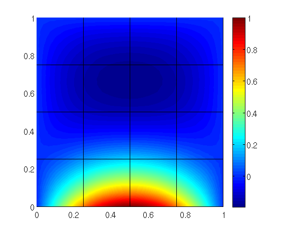
@section complete Complete Source Code
@author Dirk Klindworth, 2011
Generated on Wed Sep 13 2023 21:06:15 for Concepts by