Introduction Variational Formulation Commented Program Results References Complete Source Code
In this tutorial the implementation of the so-called BGT-0 boundary condition (Bayliss-Gunzburger-Turkel boundary condition of order 0) is shown. The BGT-0 boundary condition deals as an approximation to the Sommerfeld radiation condition of scattering problems on a disc.
The equation solved is the 2D Helmholtz equation
on the disc
with the permittivity
In the exterior domain
The coefficient functions
Now we introduce the BGT-0 boundary condition [1]
where
Finally we assume the total field
Now we derive the corresponding variational formulation of the introduced problem: find
Considering its continuity over
Using the fact that the total field in the exterior domain can be split into an incoming field and a scattered field, and incorporating the BGT-0 boundary condition gives
Now we use the continuity of the total field
Incorporating this into the variational formulation yields
Commented Program
First, system files
and concepts files
#include "basics.hh"
#include "formula.hh"
#include "function.hh"
#include "geometry.hh"
#include "graphics.hh"
#include "hp1D.hh"
#include "hp2D.hh"
#include "operator.hh"
#include "space.hh"
#include "toolbox.hh"
are included. With the following using directives
std::complex< Real > Cmplx
Type for a complex number. It also depends on the setting of Real.
we do not need to prepend concepts:: to Real and Cmplx everytime.
We start the main program
int main(int argc, char ** argv) {
try {
by setting the values of the parameters
const Real R = 15.0;
const Real innerR = 1.0;
const Real omega = 1.0;
const Real eps0 = 1.0;
const Real mu0 = 1.0;
const Cmplx epsSc (4.0, 0.0);
const Real muSc = 1.0;
and defining the attributes of the boundary, the area of the scatterer and the surrounding area respectively.
const uint attrBoundary = 11;
const uint attrSc = 21;
const uint attr0 = 22;
We specify whether the TE-case or the TM-case is computed.
enum TETM {TE, TM};
TETM mode = TM;
Then we declare PiecewiseConstFormula and ConstFormula.
We write the values of
if (mode == TE) {
alpha0 = Cmplx(pow(eps0,-1.0),0.0);
}
and in the TM-case we write
if (mode == TM) {
alpha0 = Cmplx(1.0, 0.0);
}
The wave number
const Real k0 = omega*sqrt(mu0*eps0);
in the exterior domain and the BGT-0 coefficient
const Cmplx BGTcoeff(0.0,k0);
are introduced and the incoming field ParsedFormula.
std::stringstream uIncReal, uIncImag, uIncGradReal, uIncGradImag, uIncBGTReal, uIncBGTImag;
uIncReal << "(cos((" << k0 << ")*x))" ;
uIncImag << "(sin((" << k0 << ")*x))" ;
uIncGradReal << "(-(x/(sqrt(x*x+y*y)))*" << k0 << "*sin((" << k0 << ")*x))" ;
uIncGradImag << "( (x/(sqrt(x*x+y*y)))*" << k0 << "*cos((" << k0 << ")*x))" ;
uIncBGTReal << "(" << real(BGTcoeff) << "*" << uIncReal.str() << "-" << imag(BGTcoeff) << "*" << uIncImag.str() << ")" ;
uIncBGTImag << "(" << real(BGTcoeff) << "*" << uIncImag.str() << "+" << imag(BGTcoeff) << "*" << uIncReal.str() << ")" ;
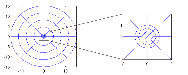
The mesh is created as a circle surrounded by a ring.
Real ringData[3] = {innerR,(innerR+R)/2.0,R};
uint quadAttrData[3] = {attrSc,attr0,attr0};
uint edgeAttrData[3] = {0,0,attrBoundary};
std::cout << std::endl << "Mesh: " << msh << std::endl;
Now the mesh is plotted using a scaling factor of 100, a greyscale of 1.0 and 20 points per edge.
MeshEPS< Real > drawMeshEPS(concepts::Mesh &msh, std::string filename, const Real scale=100, const Real greyscale=1.0, const unsigned int nPoints=2)
The space is built by refining the mesh once and setting the polynomial degree to 10. Then the elements of the space are built and the space is plotted.
spc.rebuild();
std::cout << std::endl << "Space: " << spc << std::endl;
Now the trace space of the boundary
std::cout << std::endl << "Trace Space: " << tspc << std::endl;
Set< F > makeSet(uint n, const F &first,...)
The right hand side
and the system matrix
A.addInto(S, 1.0);
M2D.addInto(S, -1.0);
M1D.addInto(S, -BGTcoeff);
std::cout << std::endl << "System Matrix: " << S << std::endl;
are computed.
We solve the equation using the direct solver SuperLU.
#endif
std::cout << std::endl << "Solver: " << solver << std::endl;
solver(rhs, sol);
In order to plot the solution the shape functions are computed on equidistant points using the trapezoidal quadrature rule.
spc.recomputeShapefunctions();
static std::unique_ptr< concepts::QuadRuleFactoryTensor2d > & factory()
Finally, exceptions are caught and a sane return value is given back.
}
std::cout << e << std::endl;
return 1;
}
#ifdef HAS_MPI
MPI_Finalize();
#endif
return 0;
}
Output of the program:
Mesh: Circle(ncell = 13, cells: Quad2d(idx = Level<2>(0, 0); 0, 0), cntr = Quad(Key(0), (Vertex(Key(0)), Vertex(Key(1)), Vertex(Key(2)), Vertex(Key(3))), Attribute(21)), vtx = [<2>(0.5, 0), <2>(0, 0.5), <2>(-0.5, 0), <2>(0, -0.5)]), Quad2d(idx = Level<2>(0, 0); 0, 0), cntr = Quad(Key(1), (Vertex(Key(1)), Vertex(Key(0)), Vertex(Key(4)), Vertex(Key(5))), Attribute(21)), vtx = [<2>(0, 0.5), <2>(0.5, 0), <2>(1, 0), <2>(0, 1)]), Quad2d(idx = Level<2>(0, 0); 0, 0), cntr = Quad(Key(2), (Vertex(Key(2)), Vertex(Key(1)), Vertex(Key(5)), Vertex(Key(6))), Attribute(21)), vtx = [<2>(-0.5, 0), <2>(0, 0.5), <2>(0, 1), <2>(-1, 0)]), Quad2d(idx = Level<2>(0, 0); 0, 0), cntr = Quad(Key(3), (Vertex(Key(3)), Vertex(Key(2)), Vertex(Key(6)), Vertex(Key(7))), Attribute(21)), vtx = [<2>(0, -0.5), <2>(-0.5, 0), <2>(-1, 0), <2>(0, -1)]), Quad2d(idx = Level<2>(0, 0); 0, 0), cntr = Quad(Key(4), (Vertex(Key(0)), Vertex(Key(3)), Vertex(Key(7)), Vertex(Key(4))), Attribute(21)), vtx = [<2>(0.5, 0), <2>(0, -0.5), <2>(0, -1), <2>(1, 0)]),
Quad2d(idx = Level<2>(0, 0); 0, 0), cntr = Quad(Key(5), (Vertex(Key(5)), Vertex(Key(4)), Vertex(Key(8)), Vertex(Key(9))), Attribute(22)), vtx = [<2>(0, 1), <2>(1, 0), <2>(8, 0), <2>(0, 8)]), Quad2d(idx = Level<2>(0, 0); 0, 0), cntr = Quad(Key(6), (Vertex(Key(6)), Vertex(Key(5)), Vertex(Key(9)), Vertex(Key(10))), Attribute(22)), vtx = [<2>(-1, 0), <2>(0, 1), <2>(0, 8), <2>(-8, 0)]), Quad2d(idx = Level<2>(0, 0); 0, 0), cntr = Quad(Key(7), (Vertex(Key(7)), Vertex(Key(6)), Vertex(Key(10)), Vertex(Key(11))), Attribute(22)), vtx = [<2>(0, -1), <2>(-1, 0), <2>(-8, 0), <2>(0, -8)]), Quad2d(idx = Level<2>(0, 0); 0, 0), cntr = Quad(Key(8), (Vertex(Key(4)), Vertex(Key(7)), Vertex(Key(11)), Vertex(Key(8))), Attribute(22)), vtx = [<2>(1, 0), <2>(0, -1), <2>(0, -8), <2>(8, 0)]), Quad2d(idx = Level<2>(0, 0); 0, 0), cntr = Quad(Key(9), (Vertex(Key(9)), Vertex(Key(8)), Vertex(Key(12)), Vertex(Key(13))), Attribute(22)), vtx = [<2>(0, 8), <2>(8, 0), <2>(15, 0), <2>(0, 15)]), Quad2d(idx = Level<2>(0, 0); 0, 0), cntr = Quad(Key(
10), (Vertex(Key(10)), Vertex(Key(9)), Vertex(Key(13)), Vertex(Key(14))), Attribute(22)), vtx = [<2>(-8, 0), <2>(0, 8), <2>(0, 15), <2>(-15, 0)]), Quad2d(idx = Level<2>(0, 0); 0, 0), cntr = Quad(Key(11), (Vertex(Key(11)), Vertex(Key(10)), Vertex(Key(14)), Vertex(Key(15))), Attribute(22)), vtx = [<2>(0, -8), <2>(-8, 0), <2>(-15, 0), <2>(0, -15)]), Quad2d(idx = Level<2>(0, 0); 0, 0), cntr = Quad(Key(12), (Vertex(Key(8)), Vertex(Key(11)), Vertex(Key(15)), Vertex(Key(12))), Attribute(22)), vtx = [<2>(8, 0), <2>(0, -8), <2>(0, -15), <2>(15, 0)]))
Space: Space(dim = 2485, nelm = 52)
Trace Space: TraceSpace(QuadEdgeFirst(), dim = 2485, nelm = 8)
System Matrix: SparseMatrix(2485x2485, HashedSparseMatrix: 228397 (3.6986%) entries bound.)
Solver: SuperLU(n = 2485)
Plot of the refined mesh:
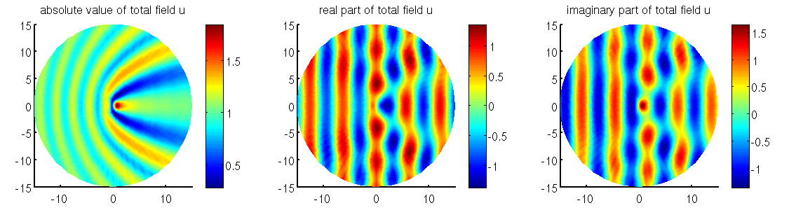
Matlab plots of the total field
[1] A. Bayliss, M. Gunzburger, and E. Turkel, "Boundary conditions for the numerical solution of elliptic equations in exterior domains", SIAM J. Appl. Math., vol. 42, no. 2, pp. 430-451, 1982.
Author Dirk Klindworth, 2011 #include <iostream>
#include "basics.hh"
#include "formula.hh"
#include "function.hh"
#include "geometry.hh"
#include "graphics.hh"
#include "hp1D.hh"
#include "hp2D.hh"
#include "operator.hh"
#include "space.hh"
#include "toolbox.hh"
int main(int argc, char ** argv) {
try {
#ifdef HAS_MPI
MPI_Init(&argc, &argv);
#endif
const Real R = 15.0;
const Real innerR = 1.0;
const Real omega = 1.0;
const Real eps0 = 1.0;
const Real mu0 = 1.0;
const Cmplx epsSc (4.0, 0.0);
const Real muSc = 1.0;
const uint attrBoundary = 11;
const uint attrSc = 21;
const uint attr0 = 22;
enum TETM {TE, TM};
TETM mode = TM;
if (mode == TE) {
alpha0 = Cmplx(pow(eps0,-1.0),0.0);
}
if (mode == TM) {
alpha0 = Cmplx(1.0, 0.0);
}
const Real k0 = omega*sqrt(mu0*eps0);
const Cmplx BGTcoeff(0.0,k0);
std::stringstream uIncReal, uIncImag, uIncGradReal, uIncGradImag, uIncBGTReal, uIncBGTImag;
uIncReal << "(cos((" << k0 << ")*x))" ;
uIncImag << "(sin((" << k0 << ")*x))" ;
uIncGradReal << "(-(x/(sqrt(x*x+y*y)))*" << k0 << "*sin((" << k0 << ")*x))" ;
uIncGradImag << "( (x/(sqrt(x*x+y*y)))*" << k0 << "*cos((" << k0 << ")*x))" ;
uIncBGTReal << "(" << real(BGTcoeff) << "*" << uIncReal.str() << "-" << imag(BGTcoeff) << "*" << uIncImag.str() << ")" ;
uIncBGTImag << "(" << real(BGTcoeff) << "*" << uIncImag.str() << "+" << imag(BGTcoeff) << "*" << uIncReal.str() << ")" ;
Real ringData[3] = {innerR,(innerR+R)/2.0,R};
uint quadAttrData[3] = {attrSc,attr0,attr0};
uint edgeAttrData[3] = {0,0,attrBoundary};
std::cout << std::endl << "Mesh: " << msh << std::endl;
std::cout << std::endl << "Space: " << spc << std::endl;
std::cout << std::endl << "Trace Space: " << tspc << std::endl;
std::cout << std::endl << "System Matrix: " << S << std::endl;
#ifdef HAS_MUMPS
#else
#endif
std::cout << std::endl << "Solver: " << solver << std::endl;
solver(rhs, sol);
std::cout << " ... solved " << std::endl;
}
std::cout << e << std::endl;
return 1;
}
#ifdef HAS_MPI
MPI_Finalize();
#endif
return 0;
}
void addInto(Matrix< H > &dest, const I fact, const uint rowoffset=0, const uint coloffset=0) const
void recomputeShapefunctions()
virtual uint dim() const
Returns the dimension of the space.
![\[
- \nabla \cdot \alpha \nabla u - \beta u = 0
\]](form_34_dark.png)


![\[
\alpha = \frac{1}{\epsilon}, \qquad \beta = \omega^2 \mu,
\]](form_42_dark.png)


![\[
\alpha \equiv 1, \qquad \beta = \omega^2 \epsilon \mu.
\]](form_46_dark.png)


![\[
u^{\rm ext} = u^{\rm inc} + u^{\rm sc}.
\]](form_51_dark.png)


![\[
\nabla u^{\rm sc} \cdot \mathbf{n} = {\rm i} k_0 u^{\rm sc}
\qquad \text{on }\partial\Omega,
\]](form_59_dark.png)


![\[
\int_{\Omega}\alpha \nabla u \cdot \nabla v\;{\rm d}\mathbf{x}
- \int_{\Omega}\beta uv\;{\rm d}\mathbf{x}
- \int_{\partial\Omega} \alpha \nabla u \cdot \mathbf{n} v \;{\rm d}s(\mathbf{x})
= 0 \qquad\forall v\in H^1(\Omega).
\]](form_65_dark.png)
![\[
\alpha\nabla u\cdot \mathbf{n}
= \alpha_0\nabla u^{\rm ext} \cdot \mathbf{n}
\qquad \text{on }\partial\Omega.
\]](form_66_dark.png)
![\[
\alpha \nabla u \cdot \mathbf{n}
= \alpha_0 \left( {\rm i}k_0u^{\rm sc}
+ \nabla u^{\rm inc} \cdot \mathbf{n}
\right)
\qquad \text{on }\partial\Omega.
\]](form_67_dark.png)
![\[
\alpha \nabla u \cdot \mathbf{n}
= \alpha_0 \left( {\rm i}k_0 u^{\rm ext}
- {\rm i}k_0 u^{\rm inc}
+ \nabla u^{\rm inc} \cdot \mathbf{n}
\right)
= \alpha_0 \left( {\rm i}k_0 u
- {\rm i}k_0 u^{\rm inc}
+ \nabla u^{\rm inc} \cdot \mathbf{n}
\right)
\qquad \text{on }\partial\Omega.
\]](form_68_dark.png)
![\[
\int_{\Omega}\alpha \nabla u \cdot \nabla v\;{\rm d}\mathbf{x}
- \int_{\Omega}\beta uv\;{\rm d}\mathbf{x}
- \alpha_0\int_{\partial\Omega} {\rm i} k_0 u \;{\rm d}s(\mathbf{x})
= \alpha_0\int_{\partial\Omega} \left(\nabla u^{\rm inc} \cdot \mathbf{n}
- {\rm i} k_0 u^{\rm inc}\right) v \;{\rm d}s(\mathbf{x})
\qquad\forall v\in H^1(\Omega).
\]](form_69_dark.png)